arviz.plot_autocorr

arviz.plot_autocorr(data, var_names=None, filter_vars=None, max_lag=None, combined=False, coords=None, grid=None, figsize=None, textsize=None, labeller=None, ax=None, backend=None, backend_config=None, backend_kwargs=None, show=None)

Bar plot of the autocorrelation function (ACF) for a sequence of data.

The ACF plots are helpful as a convergence diagnostic for posteriors from MCMC samples which display autocorrelation.

Parameters:

dataInferenceData

Any object that can be converted to an arviz.InferenceData object refer to documentation of arviz.convert_to_dataset() for details

var_nameslist of str, optional

Variables to be plotted. Prefix the variables by ~ when you want to exclude them from the plot. See this section for usage examples.

filter_vars{None, “like”, “regex”}, default None

If None (default), interpret var_names as the real variables names. If “like”, interpret var_names as substrings of the real variables names. If “regex”, interpret var_names as regular expressions on the real variables names. See this section for usage examples.

coords: mapping, optional

Coordinates of var_names to be plotted. Passed to xarray.Dataset.sel()

max_lagint, optional

Maximum lag to calculate autocorrelation. By Default, the plot displays the first 100 lag or the total number of draws, whichever is smaller.

combinedbool, default False

Flag for combining multiple chains into a single chain. If False, chains will be plotted separately.

gridtuple, optional

Number of rows and columns. Defaults to None, the rows and columns are automatically inferred. See this section for usage examples.

figsize(float, float), optional

Figure size. If None it will be defined automatically. Note this is not used if ax is supplied.

textsizefloat, optional

Text size scaling factor for labels, titles and lines. If None it will be autoscaled based on figsize.

labellerLabeller, optional

Class providing the method make_label_vert to generate the labels in the plot titles. Read the Label guide for more details and usage examples.

ax2D array_like of matplotlib Axes or Bokeh Figure, optional

A 2D array of locations into which to plot the densities. If not supplied, ArviZ will create its own array of plot areas (and return it).

backend{“matplotlib”, “bokeh”}, default “matplotlib”

Select plotting backend.

backend_configdict, optional

Currently specifies the bounds to use for bokeh axes. Defaults to value set in rcParams.

backend_kwargsdict, optional

These are kwargs specific to the backend being used, passed to matplotlib.pyplot.subplots() or bokeh.plotting.figure. For additional documentation check the plotting method of the backend.

showbool, optional

Call backend show function.

Returns:

axesmatplotlib Axes or bokeh_figures

See also

autocov

Compute autocovariance estimates for every lag for the input array.

autocorr

Compute autocorrelation using FFT for every lag for the input array.

Examples

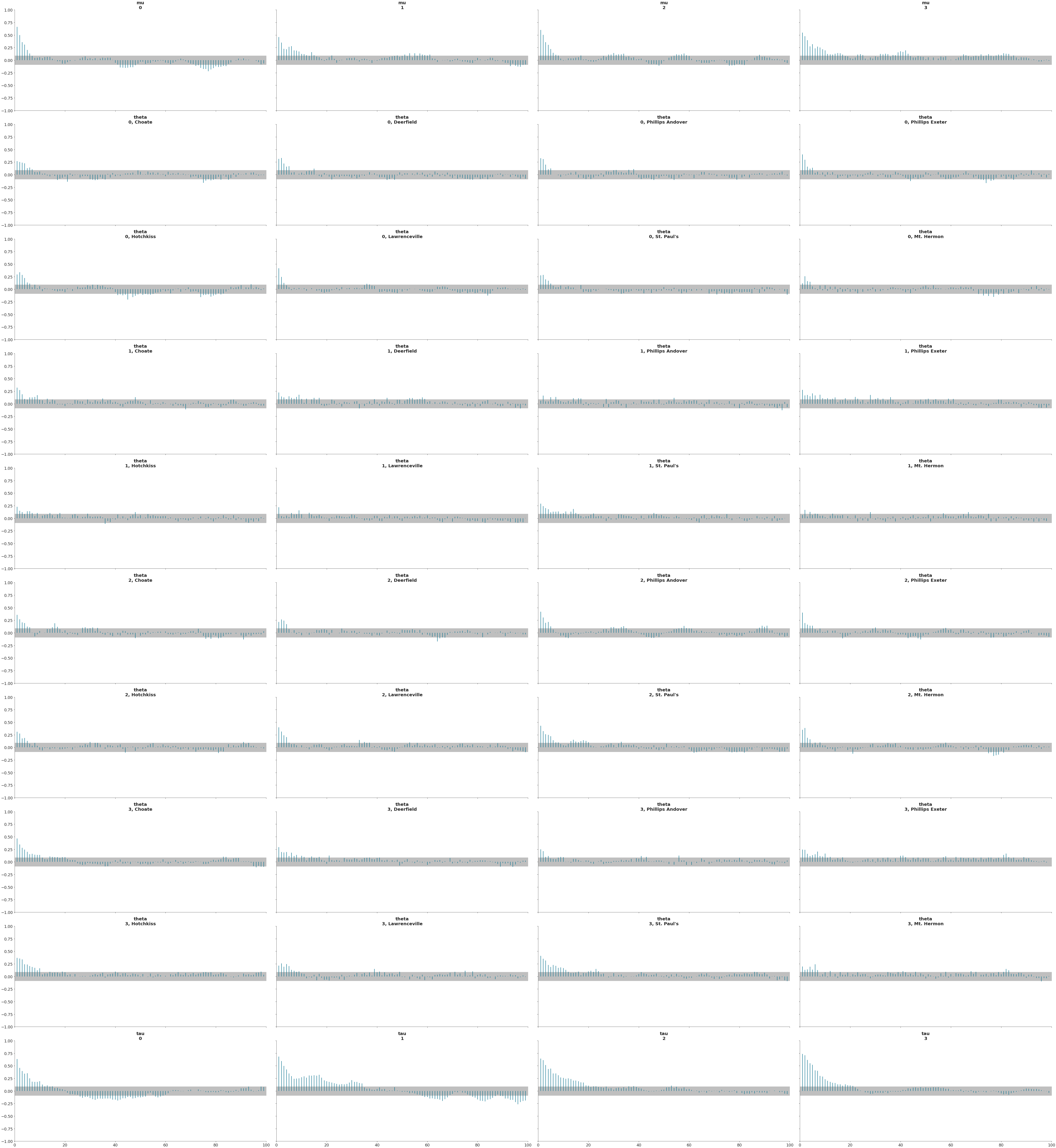
Plot default autocorrelation

>>> import arviz as az
>>> data = az.load_arviz_data('centered_eight')
>>> az.plot_autocorr(data)

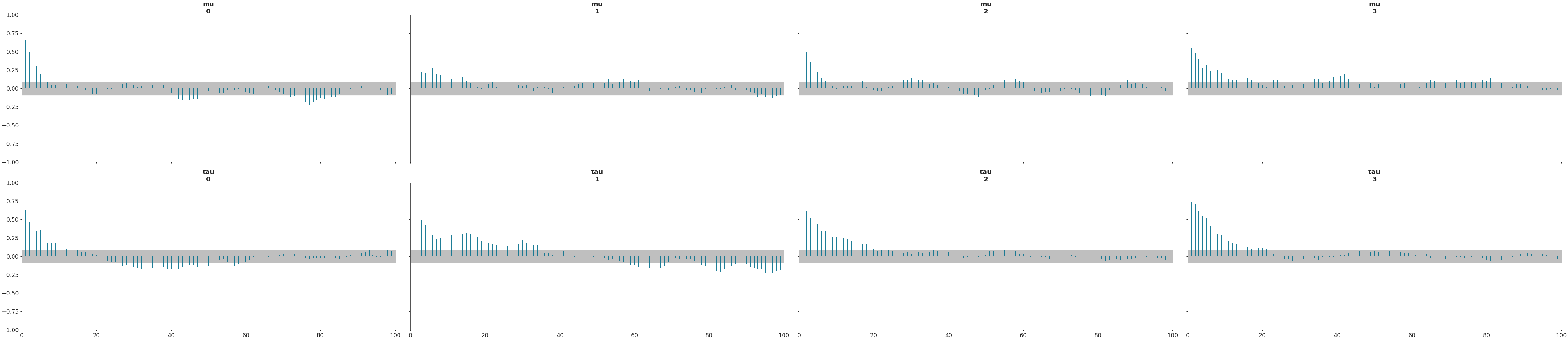
Plot subset variables by specifying variable name exactly

>>> az.plot_autocorr(data, var_names=['mu', 'tau'] )

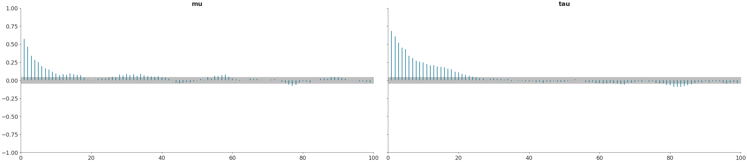
Combine chains by variable and select variables by excluding some with partial naming

>>> az.plot_autocorr(data, var_names=['~thet'], filter_vars="like", combined=True)

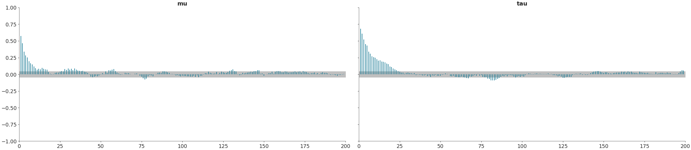
Specify maximum lag (x axis bound)

>>> az.plot_autocorr(data, var_names=['mu', 'tau'], max_lag=200, combined=True)