arviz.plot_forest#
- arviz.plot_forest(data, kind='forestplot', model_names=None, var_names=None, filter_vars=None, transform=None, coords=None, combined=False, combine_dims=None, hdi_prob=None, rope=None, quartiles=True, ess=False, r_hat=False, colors='cycle', textsize=None, linewidth=None, markersize=None, legend=True, labeller=None, ridgeplot_alpha=None, ridgeplot_overlap=2, ridgeplot_kind='auto', ridgeplot_truncate=True, ridgeplot_quantiles=None, figsize=None, ax=None, backend=None, backend_config=None, backend_kwargs=None, show=None)[source]#
Forest plot to compare HDI intervals from a number of distributions.
Generate forest or ridge plots to compare distributions from a model or list of models. Additionally, the function can display effective sample sizes (ess) and Rhats to visualize convergence diagnostics alongside the distributions.
- Parameters:
- data
InferenceData Any object that can be converted to an
arviz.InferenceDataobject Refer to documentation ofarviz.convert_to_dataset()for details.- kind{“forestplot”, “ridgeplot”}, default “forestplot”
Specify the kind of plot:
The
kind="forestplot"generates credible intervals, where the central points are the estimated posterior median, the thick lines are the central quartiles, and the thin lines represent the \(100\times(hdi\_prob)\%\) highest density intervals.The
kind="ridgeplot"option generates density plots (kernel density estimate or histograms) in the same graph. Ridge plots can be configured to have different overlap, truncation bounds and quantile markers.
- model_names
listofstr, optional List with names for the models in the list of data. Useful when plotting more that one dataset.
- var_names
listofstr, optional Variables to be plotted. Prefix the variables by
~when you want to exclude them from the plot. See this section for usage examples.- combine_dims
set_likeofstr, optional List of dimensions to reduce. Defaults to reducing only the “chain” and “draw” dimensions. See this section for usage examples.
- filter_vars{
None, “like”, “regex”}, defaultNone If
None(default), interpretvar_namesas the real variables names. If “like”, interpretvar_namesas substrings of the real variables names. If “regex”, interpretvar_namesas regular expressions on the real variables names. See this section for usage examples.- transform
callable(), optional Function to transform data (defaults to None i.e.the identity function).
- coords
dict, optional Coordinates of
var_namesto be plotted. Passed toxarray.Dataset.sel(). See this section for usage examples.- combinedbool, default
False Flag for combining multiple chains into a single chain. If False, chains will be plotted separately. See this section for usage examples.
- hdi_prob
float, default 0.94 Plots highest posterior density interval for chosen percentage of density. See this section for usage examples.
- rope
list,tupleordictionaryof {strtuplesorlists}, optional A dictionary of tuples with the lower and upper values of the Region Of Practical Equivalence. See this section for usage examples.
- quartilesbool, default
True Flag for plotting the interquartile range, in addition to the
hdi_probintervals.- r_hatbool, default
False Flag for plotting Split R-hat statistics. Requires 2 or more chains.
- essbool, default
False Flag for plotting the effective sample size.
- colors
listorstr, optional list with valid matplotlib colors, one color per model. Alternative a string can be passed. If the string is
cycle, it will automatically chose a color per model from the matplotlibs cycle. If a single color is passed, eg ‘k’, ‘C2’, ‘red’ this color will be used for all models. Defaults to ‘cycle’.- textsize
float, optional Text size scaling factor for labels, titles and lines. If
Noneit will be autoscaled based onfigsize.- linewidth
int, optional Line width throughout. If
Noneit will be autoscaled based onfigsize.- markersize
int, optional Markersize throughout. If
Noneit will be autoscaled based onfigsize.- legendbool, optional
Show a legend with the color encoded model information. Defaults to True, if there are multiple models.
- labellerLabeller, optional
Class providing the method
make_label_vertto generate the labels in the plot titles. Read the Label guide for more details and usage examples.- ridgeplot_alpha: float, optional
Transparency for ridgeplot fill. If
ridgeplot_alpha=0, border is colored by model, otherwise ablackoutline is used.- ridgeplot_overlap
float, default 2 Overlap height for ridgeplots.
- ridgeplot_kind
str, optional By default (“auto”) continuous variables are plotted using KDEs and discrete ones using histograms. To override this use “hist” to plot histograms and “density” for KDEs.
- ridgeplot_truncatebool, default
True Whether to truncate densities according to the value of
hdi_prob.- ridgeplot_quantiles
list, optional Quantiles in ascending order used to segment the KDE. Use [.25, .5, .75] for quartiles.
- figsize(
float,float), optional Figure size. If
None, it will be defined automatically.- ax
axes, optional matplotlib.axes.Axesorbokeh.plotting.Figure.- backend{“matplotlib”, “bokeh”}, default “matplotlib”
Select plotting backend.
- backend_config
dict, optional Currently specifies the bounds to use for bokeh axes. Defaults to value set in
rcParams.- backend_kwargs
dict, optional These are kwargs specific to the backend being used, passed to
matplotlib.pyplot.subplots()orbokeh.plotting.figure. For additional documentation check the plotting method of the backend.- showbool, optional
Call backend show function.
- data
- Returns:
- 1D
ndarrayofmatplotlib Axesorbokeh_figures
- 1D
See also
plot_posteriorPlot Posterior densities in the style of John K. Kruschke’s book.
plot_densityGenerate KDE plots for continuous variables and histograms for discrete ones.
summaryCreate a data frame with summary statistics.
Examples
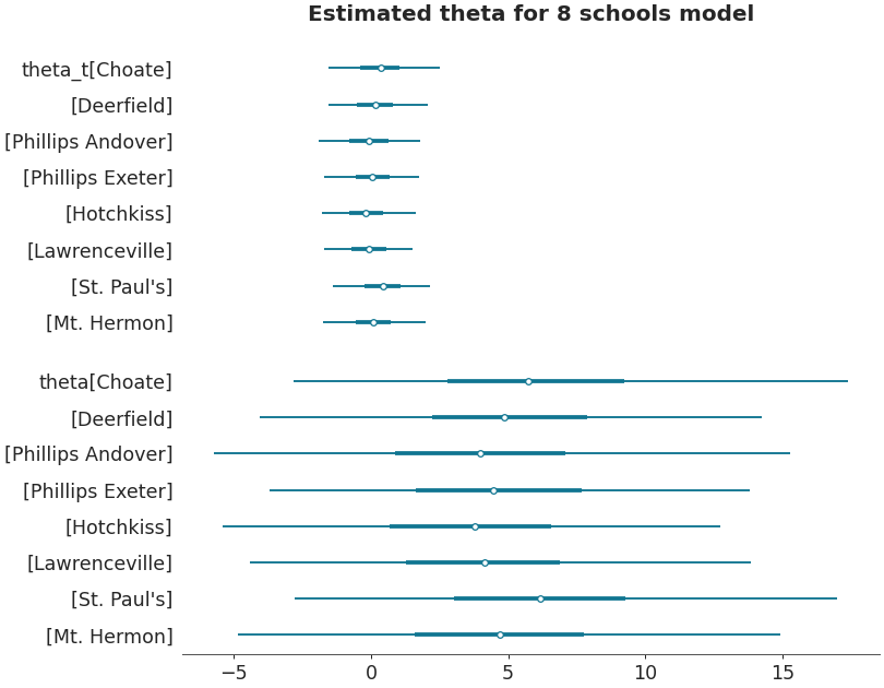
Forestplot
>>> import arviz as az
>>> non_centered_data = az.load_arviz_data('non_centered_eight')
>>> axes = az.plot_forest(non_centered_data,
>>>                            kind='forestplot',
>>>                            var_names=["^the"],
>>>                            filter_vars="regex",
>>>                            combined=True,
>>>                            figsize=(9, 7))
>>> axes[0].set_title('Estimated theta for 8 schools model')
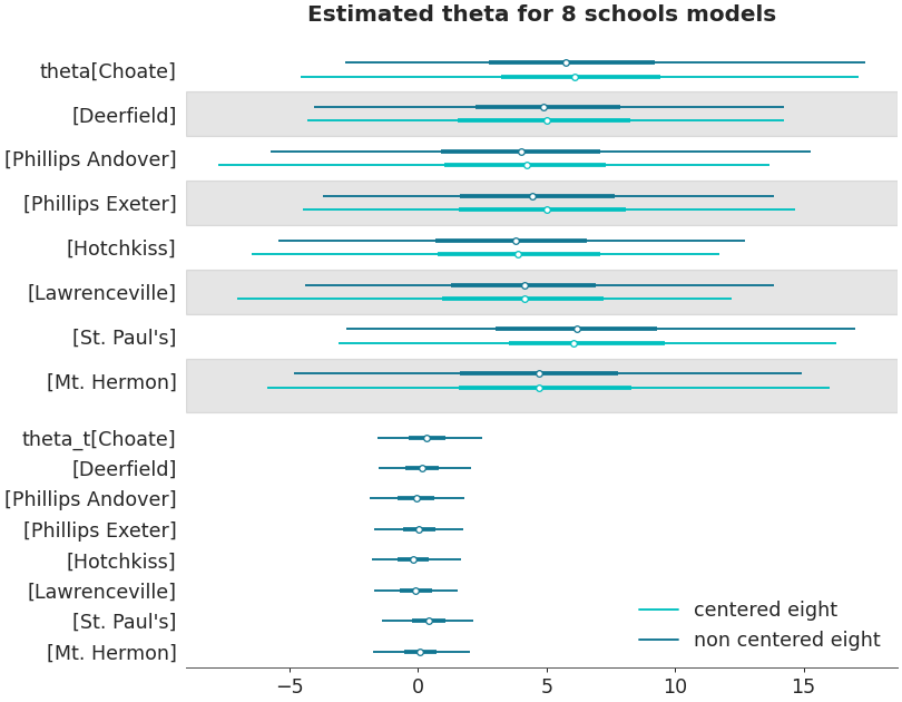
Forestplot with multiple datasets
>>> centered_data = az.load_arviz_data('centered_eight')
>>> axes = az.plot_forest([non_centered_data, centered_data],
>>>                            model_names = ["non centered eight", "centered eight"],
>>>                            kind='forestplot',
>>>                            var_names=["^the"],
>>>                            filter_vars="regex",
>>>                            combined=True,
>>>                            figsize=(9, 7))
>>> axes[0].set_title('Estimated theta for 8 schools models')
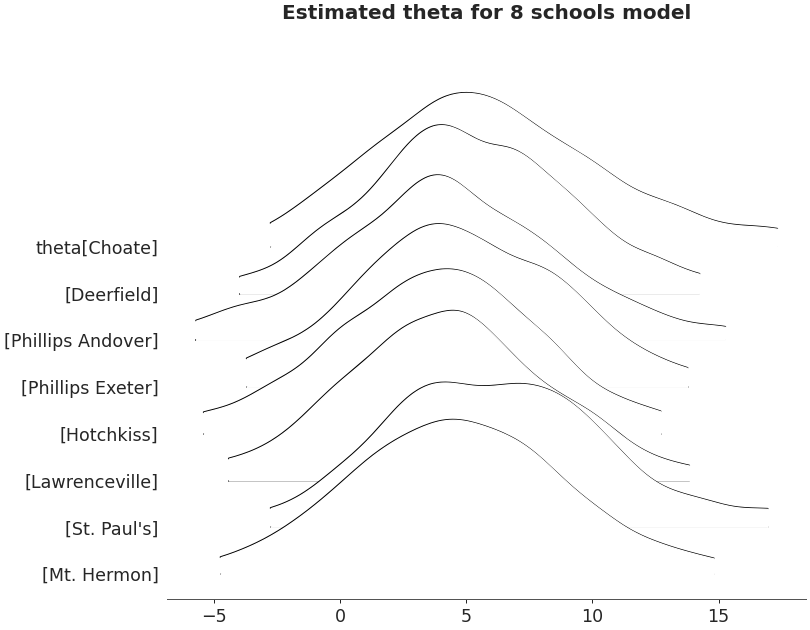
Ridgeplot
>>> axes = az.plot_forest(non_centered_data,
>>>                            kind='ridgeplot',
>>>                            var_names=['theta'],
>>>                            combined=True,
>>>                            ridgeplot_overlap=3,
>>>                            colors='white',
>>>                            figsize=(9, 7))
>>> axes[0].set_title('Estimated theta for 8 schools model')
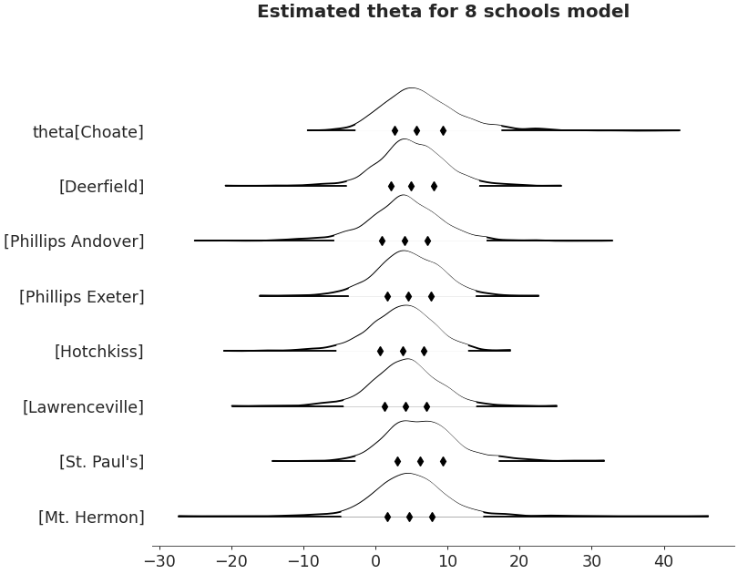
Ridgeplot non-truncated and with quantiles
>>> axes = az.plot_forest(non_centered_data,
>>>                            kind='ridgeplot',
>>>                            var_names=['theta'],
>>>                            combined=True,
>>>                            ridgeplot_truncate=False,
>>>                            ridgeplot_quantiles=[.25, .5, .75],
>>>                            ridgeplot_overlap=0.7,
>>>                            colors='white',
>>>                            figsize=(9, 7))
>>> axes[0].set_title('Estimated theta for 8 schools model')