arviz.plot_ecdf#
- arviz.plot_ecdf(values, values2=None, eval_points=None, cdf=None, difference=False, confidence_bands=False, ci_prob=None, num_trials=500, rvs=None, random_state=None, figsize=None, fill_band=True, plot_kwargs=None, fill_kwargs=None, plot_outline_kwargs=None, ax=None, show=None, backend=None, backend_kwargs=None, npoints=100, pointwise=False, fpr=None, pit=False, **kwargs)[source]#
Plot ECDF or ECDF-Difference Plot with Confidence bands.
Plots of the empirical cumulative distribution function (ECDF) of an array. Optionally, A
cdfargument representing a reference CDF may be provided for comparison using a difference ECDF plot and/or confidence bands.Alternatively, the PIT for a single dataset may be visualized.
- Parameters:
- valuesarray_like
Values to plot from an unknown continuous or discrete distribution.
- values2array_like, optional
values to compare to the original sample.
Deprecated since version 0.18.0: Instead use
cdf=scipy.stats.ecdf(values2).cdf.evaluate.- cdf
callable(), optional Cumulative distribution function of the distribution to compare the original sample. The function must take as input a numpy array of draws from the distribution.
- differencebool, default
False If True then plot ECDF-difference plot otherwise ECDF plot.
- confidence_bands
stror bool False: No confidence bands are plotted (default).
True: Plot bands computed with the default algorithm (subject to change)
“pointwise”: Compute the pointwise (i.e. marginal) confidence band.
“optimized”: Use optimization to estimate a simultaneous confidence band.
“simulated”: Use Monte Carlo simulation to estimate a simultaneous confidence band.
For simultaneous confidence bands to be correctly calibrated, provide
eval_pointsthat are not dependent on thevalues.- ci_prob
float, default 0.94 The probability that the true ECDF lies within the confidence band. If
confidence_bandsis “pointwise”, this is the marginal probability instead of the joint probability.- eval_pointsarray_like, optional
The points at which to evaluate the ECDF. If None,
npointsuniformly spaced points between the data bounds will be used.- rvs: callable, optional
A function that takes an integer
ndrawsand optionally the object passed torandom_stateand returns an array ofndrawssamples from the same distribution as the original dataset. Required ifmethodis “simulated” and variable is discrete.- random_state
int,numpy.random.Generatorornumpy.random.RandomState, optional - num_trials
int, default 500 The number of random ECDFs to generate for constructing simultaneous confidence bands (if
confidence_bandsis “simulated”).- figsize(float,float), optional
Figure size. If
Noneit will be defined automatically.- fill_bandbool, default
True If True it fills in between to mark the area inside the confidence interval. Otherwise, plot the border lines.
- plot_kwargs
dict, optional Additional kwargs passed to
matplotlib.pyplot.step()orbokeh.plotting.figure.step()- fill_kwargs
dict, optional Additional kwargs passed to
matplotlib.pyplot.fill_between()orbokeh:bokeh.plotting.Figure.varea()- plot_outline_kwargs
dict, optional Additional kwargs passed to
matplotlib.axes.Axes.plot()orbokeh:bokeh.plotting.Figure.line()- ax :axes, optional
Matplotlib axes or bokeh figures.
- showbool, optional
Call backend show function.
- backend{“matplotlib”, “bokeh”}, default “matplotlib”
Select plotting backend.
- backend_kwargs
dict, optional These are kwargs specific to the backend being used, passed to
matplotlib.pyplot.subplots()orbokeh.plotting.figure. For additional documentation check the plotting method of the backend.- npoints
int, default 100 The number of evaluation points for the ecdf or ecdf-difference plots, if
eval_pointsis not provided orpitisTrue.Deprecated since version 0.18.0: Instead specify
eval_points=np.linspace(np.min(values), np.max(values), npoints)unlesspitisTrue.- pointwisebool, default
False Deprecated since version 0.18.0: Instead use
confidence_bands="pointwise".- fpr
float, optional Deprecated since version 0.18.0: Instead use
ci_prob=1-fpr.- pitbool, default
False If True plots the ECDF or ECDF-diff of PIT of sample.
Deprecated since version 0.18.0: See below example instead.
- Returns:
- axes
matplotlib AxesorBokeh Figure
- axes
Notes
This plot computes the confidence bands with the simulated based algorithm presented in [1].
References
[1]Säilynoja, T., Bürkner, P.C. and Vehtari, A. (2022). Graphical Test for Discrete Uniformity and its Applications in Goodness of Fit Evaluation and Multiple Sample Comparison. Statistics and Computing, 32(32).
Examples
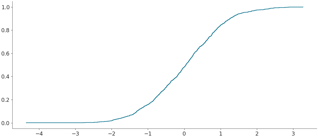
In a future release, the default behaviour of
plot_ecdfwill change. To maintain the original behaviour you should do:>>> import arviz as az >>> import numpy as np >>> from scipy.stats import uniform, norm >>> >>> sample = norm(0,1).rvs(1000) >>> npoints = 100 >>> az.plot_ecdf(sample, eval_points=np.linspace(sample.min(), sample.max(), npoints))
However, seeing this warning isn’t an indicator of anything being wrong, if you are happy to get different behaviour as ArviZ improves and adds new algorithms you can ignore it like so:
>>> import warnings
>>> warnings.filterwarnings("ignore", category=az.utils.BehaviourChangeWarning)
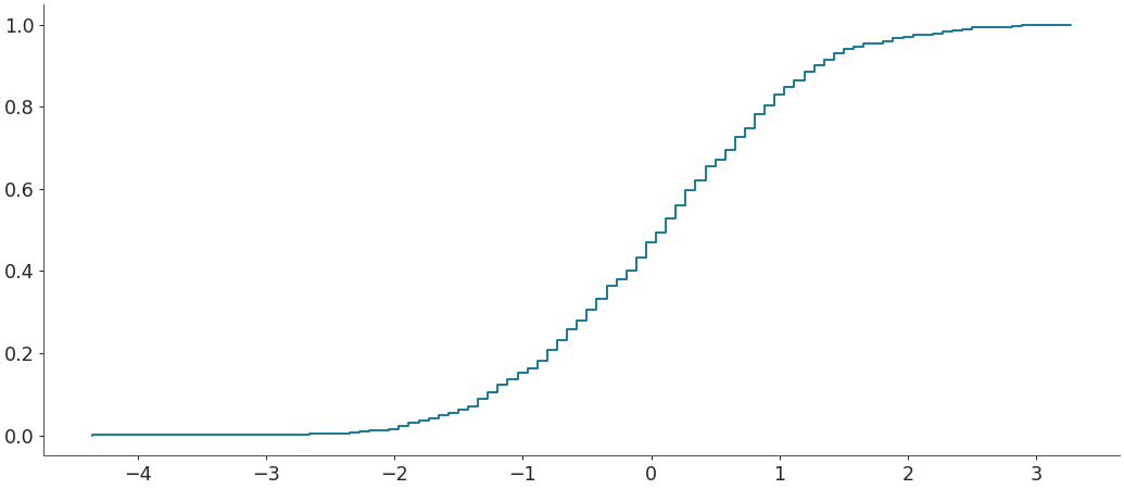
Plot an ECDF plot for a given sample evaluated at the sample points. This will become the new behaviour when
eval_pointsis not provided:>>> az.plot_ecdf(sample, eval_points=np.unique(sample))
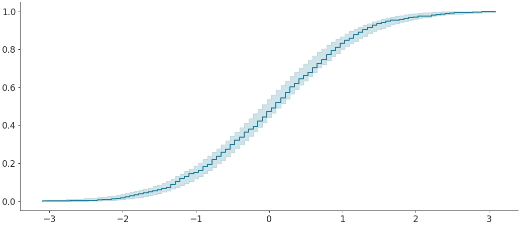
Plot an ECDF plot with confidence bands for comparing a given sample to a given distribution. We manually specify evaluation points independent of the values so that the confidence bands are correctly calibrated.
>>> distribution = norm(0,1)
>>> eval_points = np.linspace(*distribution.ppf([0.001, 0.999]), 100)
>>> az.plot_ecdf(
>>>     sample, eval_points=eval_points,
>>>     cdf=distribution.cdf, confidence_bands=True
>>> )
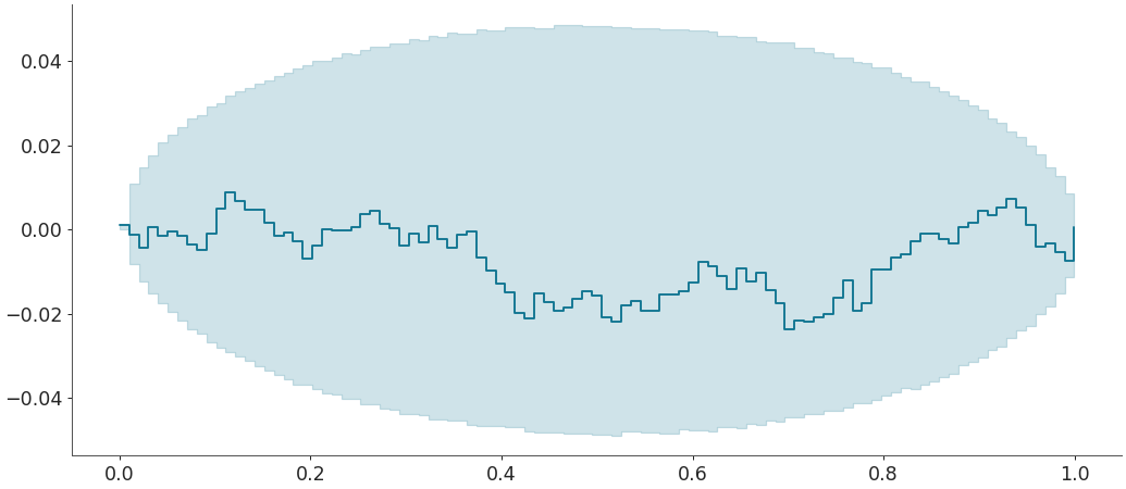
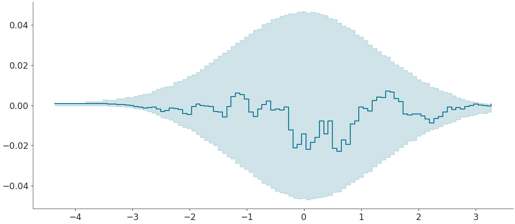
Plot an ECDF-difference plot with confidence bands for comparing a given sample to a given distribution.
>>> az.plot_ecdf(
>>>     sample, cdf=distribution.cdf,
>>>     confidence_bands=True, difference=True
>>> )
Plot an ECDF plot with confidence bands for the probability integral transform (PIT) of a continuous sample. If drawn from the reference distribution, the PIT values should be uniformly distributed.
>>> pit_vals = distribution.cdf(sample)
>>> uniform_dist = uniform(0, 1)
>>> az.plot_ecdf(
>>>     pit_vals, cdf=uniform_dist.cdf, confidence_bands=True,
>>> )

Plot an ECDF-difference plot of PIT values.
>>> az.plot_ecdf(
>>>     pit_vals, cdf = uniform_dist.cdf, confidence_bands = True,
>>>     difference = True
>>> )